A Simple Introduction to Dynamic Programming

The Optimal Decision Making Problem

Consider a situation where you have to make a series of decisions to attempt to obtain the best outcome, like, e.g., playing a game that you want to win. This is known as an optimal decision making problem or an optimal control problem.

The potential options you can choose between are called actions and the available actions are determined by the current environment or state. Once you’ve selected an action, you gain the payoff (also known as the utility or objective) associated with selecting that action in that state and then you move into the next state.

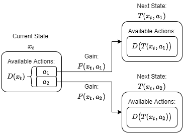
Let’s formalize this problem. We consider a discrete-time grid with a finite time-horizon, such that $t\in{0, 1, \dots, N}$. The points on this grid represent the times when we need to select an action from the set of available actions. At time $t$, we indicate the current state with $x_t$ and the set of available actions as $D(x_t)$. If we select an action, $a_t\in D(x_t)$, we gain the payoff $F(x_t, a_t)$.

We need one additional constraint, which is that the next state must only depend on the current state and the action selected. Thus, $x_{t+1} = T(x_t, a_t)$, for some function $T(x, a)$. Also note that at the final time, the end of the game, we can’t take any actions. So the payoff at the final time can only depend on the state we end up in, i.e., $F(x_N, a_N) = F(x_N)$.

The diagram below illustrates the situation where the current state $x_t$ has only two available actions, $a_1$ and $a_2$.

Figure 1. Diagram of the state space for the optimal decision making problem.

Now the optimal decision making problem becomes $V(x_t) = \max_{a_s\in D(x_s)} \sum_{s=t}^N\beta^{s-t} F(x_s, a_s).$ The goal is to maximize this value function $V$, by selecting the best possible action now and at all futures states, $a_s$ with $s=t, \dots, N$. The new addition is the discount factor, $\beta$ which is responsible for providing the present value (the value at time $t$) of the future payoffs.

If we solve this problem, we obtain two things: 1) the value of $V(x_t)$, which is the best possible present value we can get for our future actions, and 2) the series of actions themselves, the $a_s$ values for $s=t,t+1,\ldots,N,$ which tells us which actions to take to obtain this best possible payoff. The corresponding function, $a(x)$, which tells us which action to take in any state $x$, is known as the policy function.

Bellman’s Principle of Optimality

To solve this problem, we’ll break it up into smaller subproblems. Let’s separate out the first decision, i.e., the first term in the summation:

\[V(x_t) = \max_{a_t\in D(x_t)} \left\{F(x_t, a_t) + \beta \left[ \max_{a_s\in D(x_s)} \sum_{s=t+1}^N\beta^{s-(t+1)} F(x_s, a_s) \right]\right\}\]

It should be clear that the second term in this expression, the term in the square brackets, is simply $V(x_{t+1})$, the value function at the next step. Thus,

\[V(x_t) = \max_{a_t\in D(x_t)} \left\{F(x_t, a_t) + \beta V(x_{t + 1})\right\}.\]

We can simplify the expression by dropping the time subscripts and explicitly showing how the next state is attained,

\[V(x) = \max_{a\in D(x)} \left\{F(x, a) + \beta V(T(x,a))\right\}.\]

This is the famous Bellman equation and it provides a recursive definition for the value function. Bellman referred to this recursive property as the principle of optimality:

Principle of Optimality: An optimal policy has the property that whatever the initial state and initial decision are, the remaining decisions must constitute an optimal policy with regard to the state resulting from the first decision.

Finding the Optimal Policy with Dynamic Programming

Dynamic programming is a recursive method to solve these sequential decision problems by using backwards induction: we solve the problem for the last period in the sequence and then use that solution to solve the problem for the second last period and so forth, until we arrive the first period.

The Bellman equation is what allows us to do this: It says that if we have the optimal value function (for all possible states) at time $t+1$ then we can find the optimal value function at time $t$ by simply maximizing over all the actions available at time $t$.

This is a big leap! In the initial problem formulation we had to maximize over all possible actions over all future states. But now we have broken that large problem up into a sequence of smaller problems. Instead of performing one large maximization over the entire time period, we perform a series of smaller maximizations, one for each time step.