Why are Expected Returns Hard to Estimate?

I encounter two questions that the internet (specifically Stackoverflow and related sites) always seems to get wrong:

1. Why expected returns are hard to estimate.
2. The origin of the so-called “square-root” law for relating the standard deviation of returns for different periods.

This post is my attempt to settle this issue completely for myself and my students. We’ll begin with the second question.

Expected Value and Variance for Log Returns of Different Periods

Consider a log-return over the period $t$ to $T$ and it’s relation to a log return of an interval of length $\Delta t$, with $(T-t)/\Delta t=m$, then

\[\begin{align} \ln\left(\frac{S(T)}{S(t)}\right) &= \ln\left(\frac{S(t + m\Delta t)}{S(t)}\right), \\ &= \ln\left(\frac{S(t + m\Delta t)}{S(t + (m-1)\Delta t)}\cdot\frac{S(t + (m-1)\Delta t)}{S(t + (m-2)\Delta t)}\cdots\frac{S(t + 2\Delta t)}{S(t + \Delta t)}\frac{S(t + \Delta t)}{S(t)}\right), \\ &= \sum_{i=1}^m \ln\left(\frac{S(t + i\Delta t)}{S(t + (i-1)\Delta t)}\right). \end{align}\]

Let $X_T=\ln\left(\frac{S(T)}{S(t)}\right)$, be a random variable with mean $\bar{X}_T $ and variance $\sigma_T^2$.

Let $X_{i\Delta t} = \ln\left(\frac{S(t + i\Delta t)}{S(t + (i-1)\Delta t)}\right)$, be a collection of random variables (indexed by $i$), that are uncorrelated, and identically distributed, each with mean $\bar{X}_{\Delta t}$ and variance $\sigma_{\Delta t}^2$.

Since \[ X_T \overset{d}{=} \sum_{i=1}^m X_{i \Delta t}, \] we obtain

\[\begin{align} \operatorname{Var}\left(X_T\right) &= \operatorname{Var}\left(\sum_{i=1}^m X_{i \Delta t}\right) = \sum_{i=1}^m \operatorname{Var}\left(X_{i \Delta t}\right) = m\cdot \sigma_{\Delta t}^2\\ &{\text{and}} \\ \\ \operatorname{E}\left(X_T\right) &= \operatorname{E}\left(\sum_{i=1}^m X_{i \Delta t}\right) = \sum_{i=1}^m \operatorname{E}\left(X_{i \Delta t}\right) = m\cdot \bar{X}_{\Delta t}. \end{align}\]

Such that

\[\sigma^2_T = m \cdot \sigma^2_{\Delta t} \quad\text{and}\quad \bar{X}_T=m\cdot \bar{X}_{\Delta t}.\]

Note: If $T=1$ and $t=0$, such that $X_1$ is the annual return, and $\Delta t = \frac{1}{255}$ is a single trading day, we obtain the classical result that

\[\sigma_{\frac{1}{255}} = \frac{\sigma_1}{\sqrt{255}}.\]

Estimating Expected Returns

Consider that we have $N$ uncorrelated samples of $X_T$, denoted $X_T^{(i)}$ for $i=1,\dots,N$. The typical estimator for the sample mean is given by

\[\hat{\bar{X}}_T = \frac{1}{N}\sum_{i=1}^N X_T^{(i)}.\]

We want to investigate the properties of this estimator, for example, how much data would we need to have a “good” estimate? First, we consider the mean of the estimator

\[\operatorname{E}\left(\hat{\bar{X}}_T\right) = \frac{1}{N} \sum_{i=1}^N \operatorname{E}\left(X_T^{(i)}\right) = \frac{1}{N}\cdot N\cdot \bar{X}_T = \bar{X}_T.\]

Thus, this estimator is unbiased: its expected value is the true value of the parameter being estimated.

Next, we consider the variance of the estimator

\[\operatorname{Var}\left(\hat{\bar{X}}_T\right) = \operatorname{Var}\left(\frac{1}{N}\sum_{i=1}^N X_T^{(i)}\right) = \frac{1}{N^2} \operatorname{Var}\left(\sum_{i=1}^N X_T^{(i)}\right) = \frac{N}{N^2} \sigma_T^2 = \frac{\sigma_T^2}{N}.\]

On the surface, this result is not surprising: as we increase the number of samples in our data set, the variance of our mean estimator decreases, going to zero as our number of samples goes to infinity. Unfortunately, this is not great given the typical values for financial data.

Consider the case where $\bar{X}_1 = 10\%$ and $\sigma_1 = 20\%$, i.e., the expected annual return is 10% and the annual volatility is 20%. The table below shows the standard deviation of the estimator as a percentage of the true value we are trying to estimate.

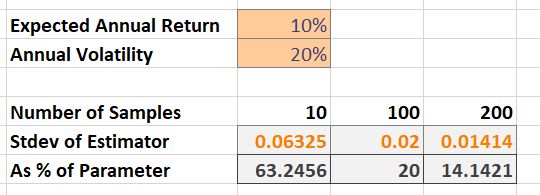
We would need at least 100 years of independent annual returns to estimate the expected return such that our estimate has a standard deviation of only 20% of the true value.

Perhaps we can improve our estimator for $X_T$ by consider returns over smaller intervals, $X_{\Delta t}$?

Note: The Bank of New York Mellon Corporation (BNY Mellon) is the longest listed company on the NYSE. It was listed in 1792. That’s the equivalent of 229 samples of annual returns ($X_1$).

Period-Length Effects for Expected Returns

We can attempt to exploit the relationship between $X_T$ and $X_{i\Delta t}$ to improve $\hat{\bar{X}}_T$. For example, if we have $N=100$ samples of annual returns ($X_1^{(i)}$), we may have access to $N\cdot m = 100 \cdot 255$ samples of daily returns ($X_{\frac{1}{255}}^{(i)}$).

We consider a new estimator for the sample mean of $X_T$, denoted $\hat{\bar{X}}^*_T$, using our samples of $X_{i \Delta t}^{(i)}$,

\[\hat{\bar{X}}^*_T := m\cdot \hat{\bar{X}}_{\Delta t} = m\frac{1}{Nm}\sum_{i=1}^{Nm} X_{i \Delta t}^{(i)} = \frac{1}{N} \sum_{i=1}^{Nm} X_{i \Delta t}^{(i)}.\]

This estimator is unbiased,

\[\operatorname{E}\left(\hat{\bar{X}}^*_T\right) = \frac{1}{N} \sum_{i=1}^{Nm} \operatorname{E}\left(X_{i\Delta t}^{(i)}\right) = \frac{Nm}{N}\bar{X}_{\Delta t} = \bar{X}_T.\]

Unfortunately, it has the same variance as the previous estimator,

\[\operatorname{Var}\left(\hat{\bar{X}}^*_T\right) = \operatorname{Var}\left(\frac{1}{N}\sum_{i=1}^{Nm} X_{i\Delta t}^{(i)}\right) = \frac{1}{N^2} \operatorname{Var}\left(\sum_{i=1}^{Nm} X_{i\Delta t}^{(i)}\right) = \frac{Nm}{N^2} \sigma_{\Delta T}^2 = \frac{\sigma_T^2}{N}.\]

Thus, our estimate for expected return cannot be improved by subdividing our interval. This is a direct result of the additive or compound nature of returns.

Estimating Variance

Consider the unbiased sample estimator for $\sigma_T^2$,

\[\hat{\sigma}^2_T = \frac{1}{N-1}\sum_{i=1}^N\left(X_T^{(i)} - \hat{\bar{X}} \right)^2.\]

IF we assume that $X_T\sim\mathcal{N}\left(\bar{X}_T,\sigma^2_T\right)$, then the variance of this estimator is given by

\[\operatorname{Var}\left(\hat{\sigma}^2_T\right) = \frac{2\sigma_T^4}{N - 1}.\]

This is already an enormous improvement on our estimate for the mean. Consider again the case where $\bar{X}_1 = 10\%$ and $\sigma_1 = 20\%$, i.e., the expected annual return is 10% and the annual volatility is 20%. The table below shows the standard deviation of the estimator as a percentage of the true value we are trying to estimate.

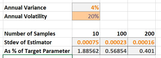
Even with only 10 samples, the standard deviation of our estimate is less than 2% of the true, target value of 4%. With an additional assumption, we can also further improve this estimate by subdividing our interval.

Period-Length Effects for Variance

We assume that the length $\Delta t$ log returns are normally distributed as well, that is, $X_{i\Delta t} \sim \mathcal{N}\left(\bar{X}_{\Delta t},\sigma^2_{\Delta t}\right).$ We consider a new estimator for the sample variance of $X_T$, denoted $\hat{\sigma}^{2,*}_T$, using our samples of $X_{i \Delta t}^{(i)}$,

\[\hat{\sigma}^{2,*}_T := m\cdot \hat{\sigma}^2_{\Delta t}\]

where $\hat{\sigma}^2_{\Delta t}$ is the standard unbiased sample estimator for the variance of $X_{i\Delta t}.$ It should immediately be clear that this estimator is unbiased. However, the variance of this new estimator becomes

\[\operatorname{Var}\left(\hat{\sigma}^{2,*}_T\right) = m^2\frac{2\sigma_{\Delta t}^4}{Nm - 1} = \frac{2\sigma^2_T}{Nm - 1}.\]

Now, the variance of the new estimator is less than the variance of the old estimator, as long as $m>1$, which occurs whenever $\Delta t < T - t$.

Thus, our estimate for variance can be improved by subdividing our interval. In fact, the more frequently we can sample our return, the better our estimate for variance.